
摘要
本篇文章深入探討穀物的營養成分與其對健康的重要影響,幫助讀者更好地理解如何選擇適合的穀物以促進身體健康。 歸納要點:
- 穀物的營養成分多樣性,特別是全穀物如糙米和燕麥,富含纖維、維生素B群及礦物質,對健康有益。
- 全穀物中的纖維能促進腸道益菌增長,有助於改善腸道健康並降低慢性疾病風險。
- 選擇低升糖指數的全穀物,例如quinoa,有助於血糖控制,並可搭配其他蛋白質來源提升營養價值。
我們在研究許多文章後,彙整重點如下
- 全穀是指稻米、小麥、玉米等穀物的可食部分,包括麩皮、胚乳和胚芽。
- 全穀相比精製穀類,保留了更多營養成分,如維生素B群、維生素E及礦物質。
- 每日建議攝取200-300克谷類食物,其中全谷物和雜豆類應占50-150克。
- 全榖雜糧如糙米飯、全麥饅頭及紅豆等可以提供多樣養分,有助於均衡飲食。
- 碳水化合物是身體主要能源,而全穀物也富含膳食纖維,有助於腸道健康。
- 中國居民膳食指南提倡主食全谷化,強調健康飲食的重要性。
在日常生活中,我們的餐桌上經常出現各式各樣的穀物,但是否選擇了對身體最有益的呢?全穀食品不僅保留了豐富的營養成分,還能讓我們攝取更足夠的膳食纖維。每天適量地增加這些天然且未經加工的食品,不但能提升飲食品質,也對長期健康大有裨益。讓我們一起從小處著手,為自己的健康加分吧!
觀點延伸比較:| 穀物類型 | 主要營養成分 | 健康益處 | 推薦攝取量 | 最新研究趨勢 |
|---|---|---|---|---|
| 全穀類(如糙米、全麥) | 維生素B群、膳食纖維、礦物質(如鐵、鎂) | 促進腸道健康,降低心血管疾病風險 | 每日50-150克全穀物 | 越來越多的研究支持全谷物的抗氧化特性 |
| 精製穀類(如白米、白麵包) | 低纖維、高升糖指數碳水化合物 | 短期能量供應,但不利於長期健康 | 建議減少攝取,若有需可適量使用作為短期補充能量的來源 | 消費者開始重視精製與非精製穀物的差異,選擇更健康的飲食方案 |
| 雜豆類(如紅豆、綠豆) | 高蛋白質、纖維及微量元素(鋅、鉀等) | 增強免疫力,有助於控制體重和改善消化系統功能 | 每日50-100克雜豆類食物最佳搭配全谷類一起攝取 | 植物基飲食風潮持續攀升,醫學界鼓勵更多人將雜豆納入日常飲食中 |
| 燕麥片/燕麥粥 | β-glucan (可溶性纖維)、抗氧化劑 | 降低膽固醇水平,改善心血管健康 | 每日30-60克通過早餐或點心形式攝取 | 許多健身專家推廣燕麥作為理想的運動前後餐選擇 |
| 玉米(整粒) | 碳水化合物、多種抗氧化劑(玉米黃質等) | 提高視力保護和抵抗自由基損害 | 每日1份約100克左右的整粒玉米或其產品 | 新興食品科技使得更多元利用玉米,例如無添加蒸煮即食產品 |
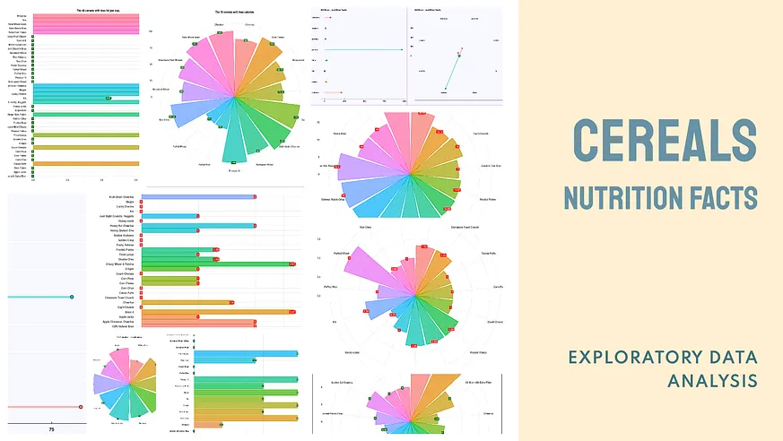
這個資料集包含80種含有營養成分的穀物。資料集80-cereals 來自Kaggle。
「如果你喜歡吃穀物,請務必避免這個資料集。看過這些資料後,我再也無法像以前那樣享受Fruity Pebbles了。」現在我們將逐步進行探索性資料分析(EDA),使用R語言。欲了解更多詳細資訊,您可以在這裡找到完整程式碼:🥣Cereals 🍎 營養 🔍 EDA 在Kaggle和🥣Cereals 🍎 營養 🔍 EDA 在GitHub上。我們需要匯入相關函式庫。
# Visualizations library(hrbrthemes) library(ggthemes) library(ggplot2) library(cowplot) # Data Manipulation library(dplyr) # Statistics library(DescTools)接著我們匯入資料,在這個案例中使用的是來自 Kaggle 的資料集,名為 80-cereals。此程式碼將顯示資料框架作為輸出。
data <- read.csv("../input/80-cereals/cereal.csv", stringsAsFactors = FALSE) # Viewing the first 6 DataFrame records head(data, 6)移除負面資料,將資料轉換以便公平地比較所有的穀物以杯為單位。
summary(data)name mfr type calories Length:77 Length:77 Length:77 Min. : 50.0 Class :character Class :character Class :character 1st Qu.:100.0 Mode :character Mode :character Mode :character Median :110.0 Mean :106.9 3rd Qu.:110.0 Max. :160.0 protein fat sodium fiber Min. :1.000 Min. :0.000 Min. : 0.0 Min. : 0.000 1st Qu.:2.000 1st Qu.:0.000 1st Qu.:130.0 1st Qu.: 1.000 Median :3.000 Median :1.000 Median :180.0 Median : 2.000 Mean :2.545 Mean :1.013 Mean :159.7 Mean : 2.152 3rd Qu.:3.000 3rd Qu.:2.000 3rd Qu.:210.0 3rd Qu.: 3.000 Max. :6.000 Max. :5.000 Max. :320.0 Max. :14.000 carbo sugars potass vitamins Min. :-1.0 Min. :-1.000 Min. : -1.00 Min. : 0.00 1st Qu.:12.0 1st Qu.: 3.000 1st Qu.: 40.00 1st Qu.: 25.00 Median :14.0 Median : 7.000 Median : 90.00 Median : 25.00 Mean :14.6 Mean : 6.922 Mean : 96.08 Mean : 28.25 3rd Qu.:17.0 3rd Qu.:11.000 3rd Qu.:120.00 3rd Qu.: 25.00 Max. :23.0 Max. :15.000 Max. :330.00 Max. :100.00 shelf weight cups rating Min. :1.000 Min. :0.50 Min. :0.250 Min. :18.04 1st Qu.:1.000 1st Qu.:1.00 1st Qu.:0.670 1st Qu.:33.17 Median :2.000 Median :1.00 Median :0.750 Median :40.40 Mean :2.208 Mean :1.03 Mean :0.821 Mean :42.67 3rd Qu.:3.000 3rd Qu.:1.00 3rd Qu.:1.000 3rd Qu.:50.83 Max. :3.000 Max. :1.50 Max. :1.500 Max. :93.70我個人認為負的營養值是不可能的,但如果我錯了,請告訴我😉
data <- subset(data,carbo >= 0) data <- subset(data,sugars >= 0) data <- subset(data,potass >= 0) summary(data)name mfr type calories Length:74 Length:74 Length:74 Min. : 50 Class :character Class :character Class :character 1st Qu.:100 Mode :character Mode :character Mode :character Median :110 Mean :107 3rd Qu.:110 Max. :160 protein fat sodium fiber carbo Min. :1.000 Min. :0 Min. : 0.0 Min. : 0.000 Min. : 5.00 1st Qu.:2.000 1st Qu.:0 1st Qu.:135.0 1st Qu.: 0.250 1st Qu.:12.00 Median :2.500 Median :1 Median :180.0 Median : 2.000 Median :14.50 Mean :2.514 Mean :1 Mean :162.4 Mean : 2.176 Mean :14.73 3rd Qu.:3.000 3rd Qu.:1 3rd Qu.:217.5 3rd Qu.: 3.000 3rd Qu.:17.00 Max. :6.000 Max. :5 Max. :320.0 Max. :14.000 Max. :23.00 sugars potass vitamins shelf Min. : 0.000 Min. : 15.00 Min. : 0.00 Min. :1.000 1st Qu.: 3.000 1st Qu.: 41.25 1st Qu.: 25.00 1st Qu.:1.250 Median : 7.000 Median : 90.00 Median : 25.00 Median :2.000 Mean : 7.108 Mean : 98.51 Mean : 29.05 Mean :2.216 3rd Qu.:11.000 3rd Qu.:120.00 3rd Qu.: 25.00 3rd Qu.:3.000 Max. :15.000 Max. :330.00 Max. :100.00 Max. :3.000 weight cups rating Min. :0.500 Min. :0.2500 Min. :18.04 1st Qu.:1.000 1st Qu.:0.6700 1st Qu.:32.45 Median :1.000 Median :0.7500 Median :40.25 Mean :1.031 Mean :0.8216 Mean :42.37 3rd Qu.:1.000 3rd Qu.:1.0000 3rd Qu.:50.52 Max. :1.500 Max. :1.5000 Max. :93.70將所有部分轉換為杯的單位
serving_onecup <- data.frame(cereal = data$name, calories = round((data$calories/(data$cups*100)*100),2), protein = round((data$protein/(data$cups*100)*100),2), fat = round((data$fat/(data$cups*100)*100),2), carbo = round((data$carbo/(data$cups*100)*100),2), fiber = round((data$fiber/(data$cups*100)*100),2), sugars = round((data$sugars/(data$cups*100)*100),2), potass = round((data$potass/(data$cups*100)*100),2), vitamins = round((data$vitamins/(data$cups*100)*100),2) ) serving_onecup <- serving_onecup[order(serving_onecup$calories, decreasing=TRUE), ] head(serving_onecup,6)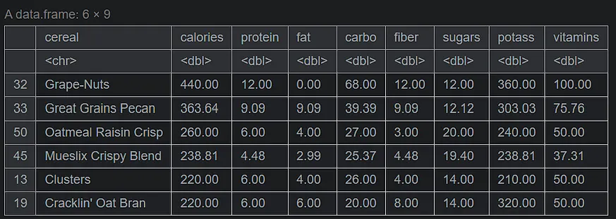
summary(serving_onecup) cereal calories protein fat Length:74 Min. : 50.0 Min. : 0.750 Min. :0.000 Class :character 1st Qu.:110.0 1st Qu.: 2.000 1st Qu.:0.000 Mode :character Median :134.3 Median : 3.000 Median :1.000 Mean :143.9 Mean : 3.587 Mean :1.425 3rd Qu.:160.0 3rd Qu.: 4.480 3rd Qu.:2.000 Max. :440.0 Max. :12.120 Max. :9.090 carbo fiber sugars potass Min. : 8.00 Min. : 0.000 Min. : 0.00 Min. : 15.0 1st Qu.:15.00 1st Qu.: 0.250 1st Qu.: 3.00 1st Qu.: 47.5 Median :17.41 Median : 2.000 Median :11.00 Median : 95.0 Mean :19.32 Mean : 3.657 Mean : 9.45 Mean :152.7 3rd Qu.:21.83 3rd Qu.: 4.000 3rd Qu.:13.40 3rd Qu.:205.2 Max. :68.00 Max. :30.300 Max. :20.90 Max. :969.7 vitamins Min. : 0.00 1st Qu.: 25.00 Median : 33.33 Mean : 38.05 3rd Qu.: 37.31 Max. :133.33 我們進行的探索性資料分析 (EDA) 專注於每杯的卡路里、脂肪、碳水化合物、纖維和糖分。為了便於展示每卡路里的資料,我們需要對卡路里進行排序,然後將資料分為上半部和下半部。
#sorting by calories serving_onecup <- serving_onecup[order(serving_onecup$calories, decreasing=TRUE), ] head(serving_onecup,6)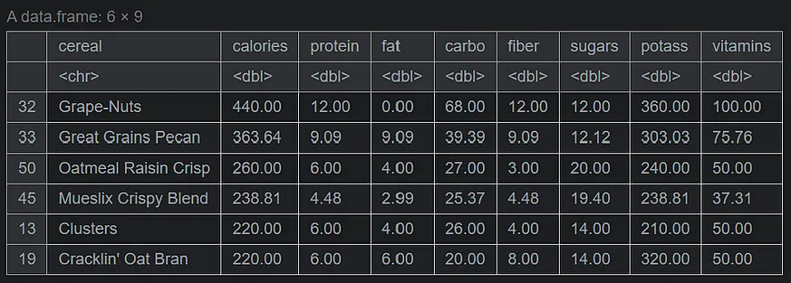
資料視覺化宣告
#Data Visualization size options(repr.plot.width = 20, repr.plot.height = 20) #higher calorie cereals df <- head(serving_onecup, 15) top_cal <- ggplot(data = df, mapping = aes(x = cereal, y = calories)) + geom_bar(stat = "identity", mapping = aes(fill = cereal, color = cereal), alpha = .7, size = 1.1) + geom_label(mapping = aes(label=calories), fill = "red", size = 6, color = "white", fontface = "bold", hjust=.7) + ggtitle("The 15 cereals with most calories") + xlab(" ") + ylab("") + theme_ipsum() + coord_flip() + theme(plot.background = element_rect(color = "black", size = 1.1), plot.title = element_text(size = 24, hjust = .5, face = "bold"), axis.title.x = element_text(size = 24, hjust = .5, face = "italic"), axis.title.y = element_text(size = 24, hjust = .5, face = "italic"), axis.text.x = element_text(size = 20, face = "bold"), axis.text.y = element_text(size = 20, face = "bold"), legend.position = "none") #low calorie cereals df1 <- tail(serving_onecup, 15) bot_cal <- ggplot(data = df1, mapping = aes(x = cereal, y = calories)) + geom_bar(stat = "identity", mapping = aes(fill = cereal, color = cereal), alpha = .7, size = 1.1) + geom_label(mapping = aes(label=calories), fill = "#006400", size = 6, color = "white", fontface = "bold", hjust=.7) + ggtitle("The 15 cereals with less calories") + xlab(" ") + ylab("") + theme_ipsum() + coord_flip() + theme(plot.background = element_rect(color = "black", size = 1.1), plot.title = element_text(size = 24, hjust = .5, face = "bold"), axis.title.x = element_text(size = 24, hjust = .5, face = "italic"), axis.title.y = element_text(size = 24, hjust = .5, face = "italic"), axis.text.x = element_text(size = 20, face = "bold"), axis.text.y = element_text(size = 20, face = "bold"), legend.position = "none")我們繪製資料視覺化圖表。
plot(top_cal+ coord_polar())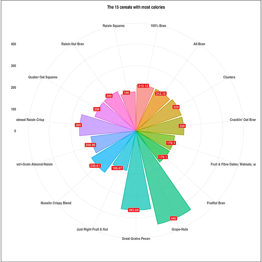
plot(bot_cal+ coord_polar())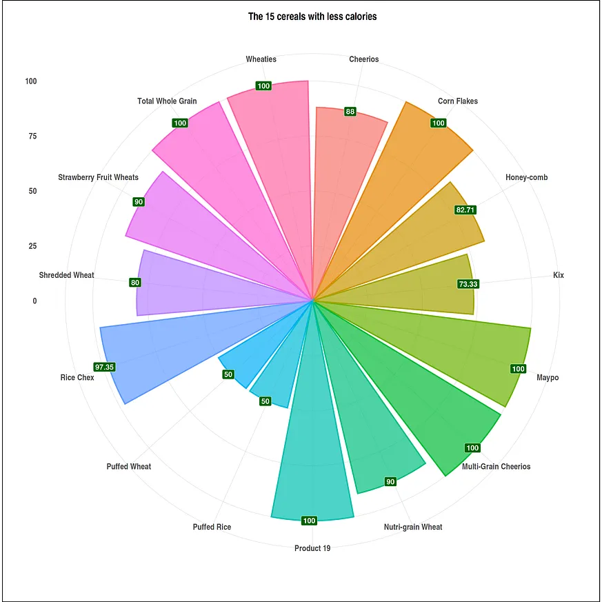
為了便於顯示每種蛋白質的資料,我們將資料按蛋白質進行降序排序,然後拆分出頭部和尾部。
#sorting by protein serving_onecup <- serving_onecup[order(serving_onecup$protein, decreasing=TRUE), ] head(serving_onecup,6)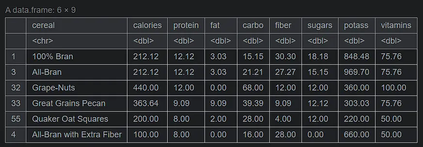
資料視覺化宣告
#size of the visuals options(repr.plot.width = 20, repr.plot.height = 20) #top of the data (cereals with more protein per cup) df <- head(serving_onecup, 15) top_protein <- ggplot(data = df, mapping = aes(x = cereal, y = protein)) + geom_bar(stat = "identity", mapping = aes(fill = cereal, color = cereal), alpha = .7, size = 1.1) + geom_label(mapping = aes(label=protein), fill = "#006400", size = 6, color = "white", fontface = "bold", hjust=.7) + ggtitle("Top 15 high protein cereals per cup.") + xlab(" ") + ylab("") + theme_ipsum() + coord_flip() + theme(plot.background = element_rect(color = "black", size = 1.1), plot.title = element_text(size = 24, hjust = .5, face = "bold"), axis.title.x = element_text(size = 24, hjust = .5, face = "italic"), axis.title.y = element_text(size = 24, hjust = .5, face = "italic"), axis.text.x = element_text(size = 20, face = "bold"), axis.text.y = element_text(size = 20, face = "bold"), legend.position = "none") #tatil of the data (cereals with less protein per cup) df1 <- tail(serving_onecup, 15) bottom_protein <- ggplot(data = df1, mapping = aes(x = cereal, y = protein)) + geom_bar(stat = "identity", mapping = aes(fill = cereal, color = cereal), alpha = .7, size = 1.1) + geom_label(mapping = aes(label=protein), fill = "red", size = 6, color = "white", fontface = "bold", hjust=.7) + ggtitle("The 15 less protein cereals per cup.") + xlab(" ") + ylab("") + theme_ipsum() + coord_flip() + theme(plot.background = element_rect(color = "black", size = 1.1), plot.title = element_text(size = 24, hjust = .5, face = "bold"), axis.title.x = element_text(size = 24, hjust = .5, face = "italic"), axis.title.y = element_text(size = 24, hjust = .5, face = "italic"), axis.text.x = element_text(size = 20, face = "bold"), axis.text.y = element_text(size = 20, face = "bold"), legend.position = "none")並且我們繪製資料視覺化圖表。
plot(top_protein+ coord_polar())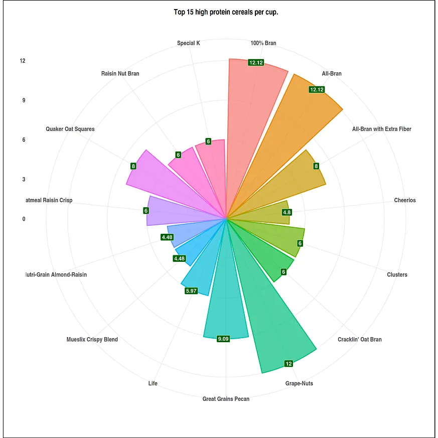
plot(bottom_protein+ coord_polar())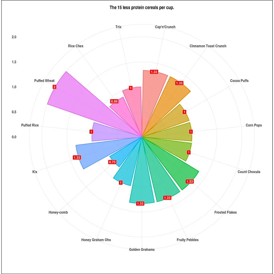
現在我們按照脂肪含量進行降序排序,然後分割出頭部和尾部。
# sorting by fat serving_onecup <- serving_onecup[order(serving_onecup$fat, decreasing=TRUE), ] head(serving_onecup,6)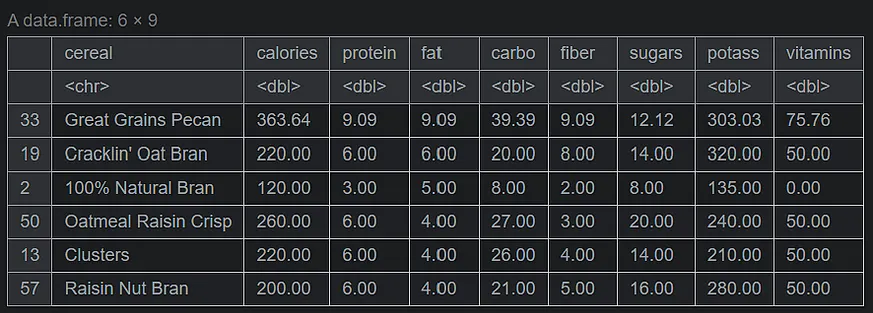
資料視覺化宣言
#visual size options(repr.plot.width = 20, repr.plot.height = 20) #data with more fat per cup df <- head(serving_onecup, 15) top_fat <- ggplot(data = df, mapping = aes(x = cereal, y = fat)) + geom_bar(stat = "identity", mapping = aes(fill = cereal, color = cereal), alpha = .7, size = 1.1) + geom_label(mapping = aes(label=fat), fill = "red", size = 6, color = "white", fontface = "bold", hjust=.7) + ggtitle("The 15 cereals with most fat per cup.") + xlab(" ") + ylab("") + theme_ipsum() + coord_flip() + theme(plot.background = element_rect(color = "black", size = 1.1), plot.title = element_text(size = 24, hjust = .5, face = "bold"), axis.title.x = element_text(size = 24, hjust = .5, face = "italic"), axis.title.y = element_text(size = 24, hjust = .5, face = "italic"), axis.text.x = element_text(size = 20, face = "bold"), axis.text.y = element_text(size = 20, face = "bold"), legend.position = "none") #data with less fat per cup df1 <- tail(serving_onecup, 40) bottom_fat <- ggplot(data = df1, mapping = aes(x = cereal, y = fat)) + geom_bar(stat = "identity", mapping = aes(fill = cereal, color = cereal), alpha = .7, size = 1.1) + geom_label(mapping = aes(label=fat), fill = "#006400", size = 6, color = "white", fontface = "bold", hjust=.7) + ggtitle("The 40 cereals with less fat per cup.") + xlab(" ") + ylab("") + theme_ipsum() + coord_flip() + theme(plot.background = element_rect(color = "black", size = 1.1), plot.title = element_text(size = 24, hjust = .5, face = "bold"), axis.title.x = element_text(size = 24, hjust = .5, face = "italic"), axis.title.y = element_text(size = 24, hjust = .5, face = "italic"), axis.text.x = element_text(size = 20, face = "bold"), axis.text.y = element_text(size = 20, face = "bold"), legend.position = "none")我們會對資料進行視覺化處理。
plot(top_fat+ coord_polar())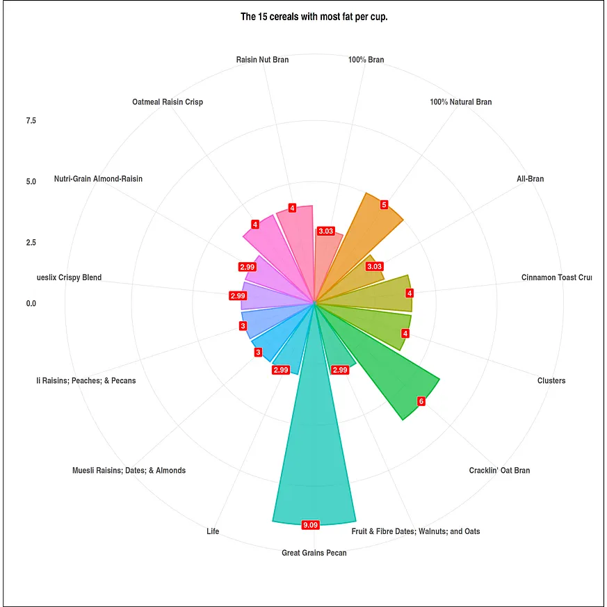
plot(bottom_fat)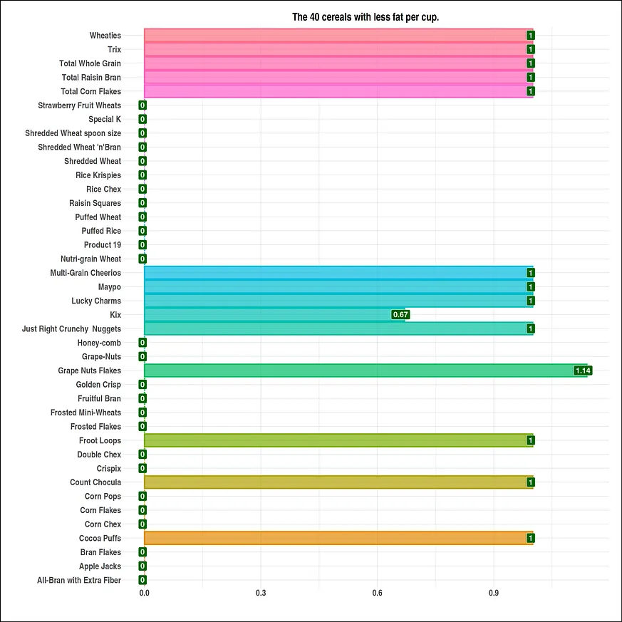
現在我們將資料按碳水化合物含量進行降序排序,然後再分割出頭部和尾部。
# sorting by carbs serving_onecup <- serving_onecup[order(serving_onecup$carbo, decreasing=TRUE), ] head(serving_onecup,6)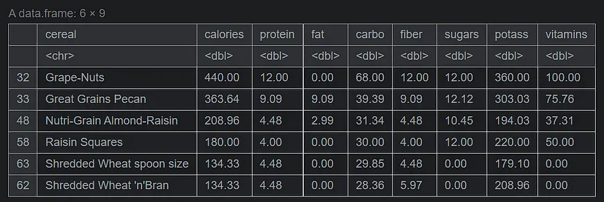
資料視覺化宣告
#visuals size options(repr.plot.width = 20, repr.plot.height = 20) #High carb data df <- head(serving_onecup, 10) top_carbo <- ggplot(data = df, mapping = aes(x = cereal, y = carbo)) + geom_bar(stat = "identity", mapping = aes(fill = cereal, color = cereal), alpha = .7, size = 1.1) + geom_label(mapping = aes(label=carbo), fill = "red", size = 6, color = "white", fontface = "bold", hjust=.7) + ggtitle("The 10 cereals with most carbs per cup") + xlab(" ") + ylab("") + theme_ipsum() + coord_flip() + theme(plot.background = element_rect(color = "black", size = 1.1), plot.title = element_text(size = 24, hjust = .5, face = "bold"), axis.title.x = element_text(size = 24, hjust = .5, face = "italic"), axis.title.y = element_text(size = 24, hjust = .5, face = "italic"), axis.text.x = element_text(size = 20, face = "bold"), axis.text.y = element_text(size = 20, face = "bold"), legend.position = "none") #low carb data df1 <- tail(serving_onecup, 10) bottom_carbo <- ggplot(data = df1, mapping = aes(x = cereal, y = carbo)) + geom_bar(stat = "identity", mapping = aes(fill = cereal, color = cereal), alpha = .7, size = 1.1) + geom_label(mapping = aes(label=carbo), fill = "#006400", size = 6, color = "white", fontface = "bold", hjust=.7) + ggtitle("The 10 cereals with less carbs per cup") + xlab(" ") + ylab("") + theme_ipsum() + coord_flip() + theme(plot.background = element_rect(color = "black", size = 1.1), plot.title = element_text(size = 24, hjust = .5, face = "bold"), axis.title.x = element_text(size = 24, hjust = .5, face = "italic"), axis.title.y = element_text(size = 24, hjust = .5, face = "italic"), axis.text.x = element_text(size = 20, face = "bold"), axis.text.y = element_text(size = 20, face = "bold"), legend.position = "none")我們將資料視覺化進行繪圖。
plot(top_carbo+ coord_polar())
plot(bottom_carbo+ coord_polar())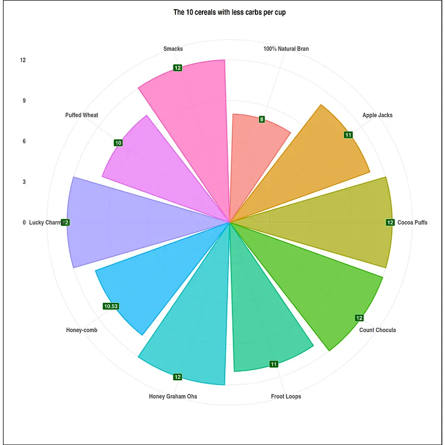
現在我們按纖維數量進行降序排序,然後分割出頭部和尾部。
# sorting by fiber serving_onecup <- serving_onecup[order(serving_onecup$fiber, decreasing=TRUE), ] head(serving_onecup,6)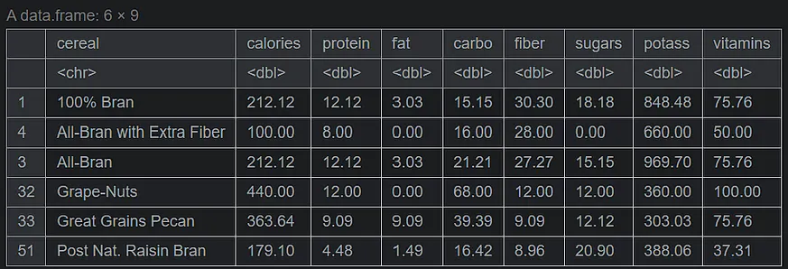
資料視覺化宣告。
#Visuals size options(repr.plot.width = 20, repr.plot.height = 20) #high fiber data df <- head(serving_onecup, 10) top_fiber <- ggplot(data = df, mapping = aes(x = cereal, y = fiber)) + geom_bar(stat = "identity", mapping = aes(fill = cereal, color = cereal), alpha = .7, size = 1.1) + geom_label(mapping = aes(label=fiber), fill = "#006400", size = 6, color = "white", fontface = "bold", hjust=.7) + ggtitle("Top 10 high fiber cereals per cup.") + xlab(" ") + ylab("") + theme_ipsum() + coord_flip() + theme(plot.background = element_rect(color = "black", size = 1.1), plot.title = element_text(size = 24, hjust = .5, face = "bold"), axis.title.x = element_text(size = 24, hjust = .5, face = "italic"), axis.title.y = element_text(size = 24, hjust = .5, face = "italic"), axis.text.x = element_text(size = 20, face = "bold"), axis.text.y = element_text(size = 20, face = "bold"), legend.position = "none") #low fiber data df1 <- tail(serving_onecup, 40) bottom_fiber <- ggplot(data = df1, mapping = aes(x = cereal, y = fiber)) + geom_bar(stat = "identity", mapping = aes(fill = cereal, color = cereal), alpha = .7, size = 1.1) + geom_label(mapping = aes(label=fiber), fill = "red", size = 6, color = "white", fontface = "bold", hjust=.7) + ggtitle("The 40 less fiber cereals per cup.") + xlab(" ") + ylab("") + theme_ipsum() + coord_flip() + theme(plot.background = element_rect(color = "black", size = 1.1), plot.title = element_text(size = 24, hjust = .5, face = "bold"), axis.title.x = element_text(size = 24, hjust = .5, face = "italic"), axis.title.y = element_text(size = 24, hjust = .5, face = "italic"), axis.text.x = element_text(size = 20, face = "bold"), axis.text.y = element_text(size = 20, face = "bold"), legend.position = "none")我們繪製資料視覺化圖表。
plot(top_fiber+ coord_polar())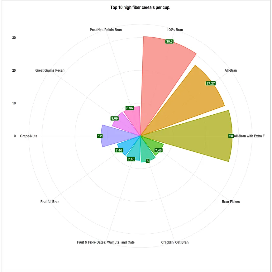
plot(bottom_fiber)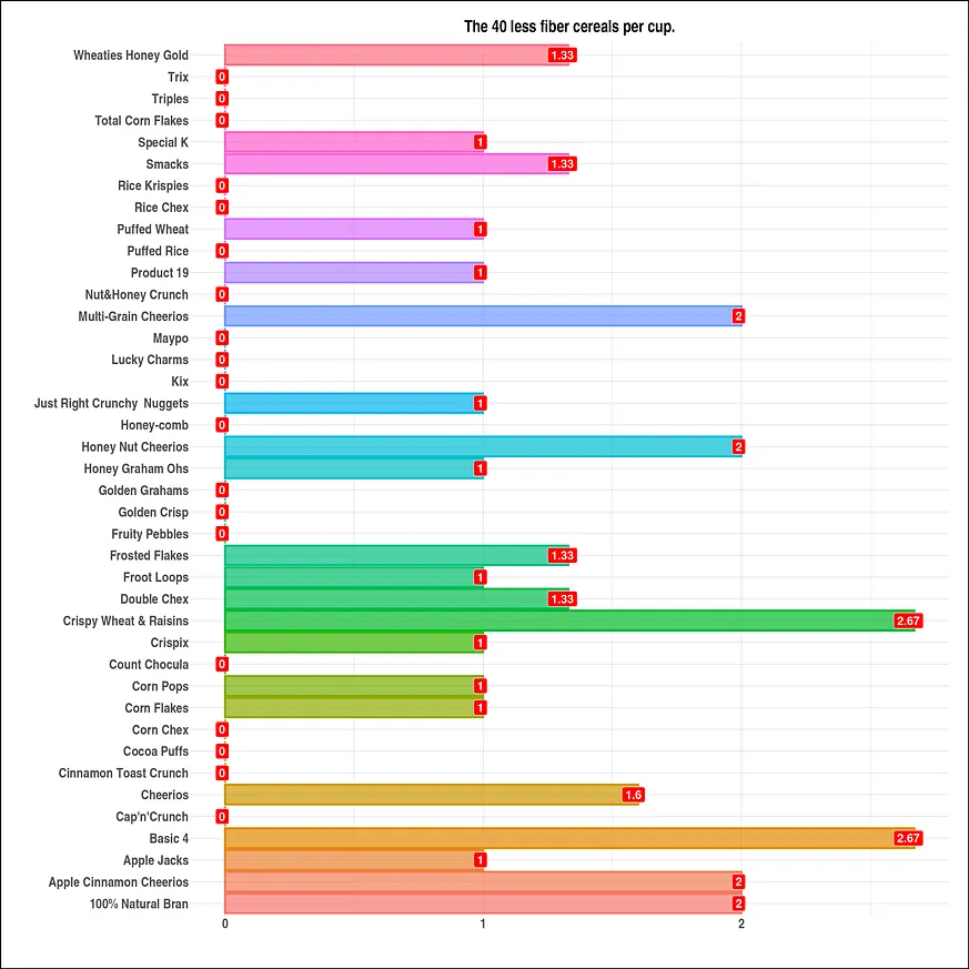
現在我們將資料依照糖分進行降序排序,然後再劃分出前端與尾端的資料。
# sorting by sugar serving_onecup <- serving_onecup[order(serving_onecup$sugars, decreasing=TRUE), ] head(serving_onecup,16)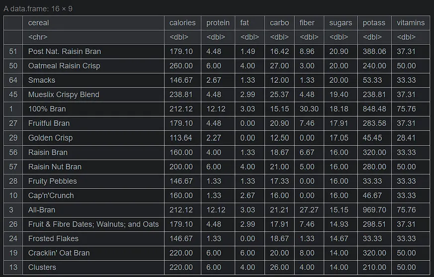
資料視覺化宣言
#visual size options(repr.plot.width = 20, repr.plot.height = 20) #High sugar data df <- head(serving_onecup, 15) top_sugar <- ggplot(data = df, mapping = aes(x = cereal, y = sugars)) + geom_bar(stat = "identity", mapping = aes(fill = cereal, color = cereal), alpha = .7, size = 1.1) + geom_label(mapping = aes(label=sugars), fill = "red", size = 6, color = "white", fontface = "bold", hjust=.7) + ggtitle("The 15 cereals with most sugar per cup.") + xlab(" ") + ylab("") + theme_ipsum() + coord_flip() + theme(plot.background = element_rect(color = "black", size = 1.1), plot.title = element_text(size = 24, hjust = .5, face = "bold"), axis.title.x = element_text(size = 24, hjust = .5, face = "italic"), axis.title.y = element_text(size = 24, hjust = .5, face = "italic"), axis.text.x = element_text(size = 20, face = "bold"), axis.text.y = element_text(size = 20, face = "bold"), legend.position = "none") #low sugar data df1 <- tail(serving_onecup, 20) bottom_sugar <- ggplot(data = df1, mapping = aes(x = cereal, y = sugars)) + geom_bar(stat = "identity", mapping = aes(fill = cereal, color = cereal), alpha = .7, size = 1.1) + geom_label(mapping = aes(label=sugars), fill = "#006400", size = 6, color = "white", fontface = "bold", hjust=.7) + ggtitle("The 20 cereals with less sugar per cup.") + xlab(" ") + ylab("") + theme_ipsum() + coord_flip() + theme(plot.background = element_rect(color = "black", size = 1.1), plot.title = element_text(size = 24, hjust = .5, face = "bold"), axis.title.x = element_text(size = 24, hjust = .5, face = "italic"), axis.title.y = element_text(size = 24, hjust = .5, face = "italic"), axis.text.x = element_text(size = 20, face = "bold"), axis.text.y = element_text(size = 20, face = "bold"), legend.position = "none")我們會繪製資料視覺化圖表。
plot(top_sugar+ coord_polar())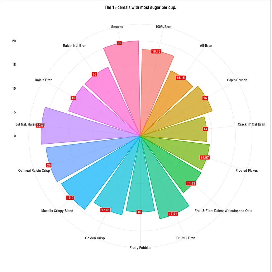
plot(bottom_sugar)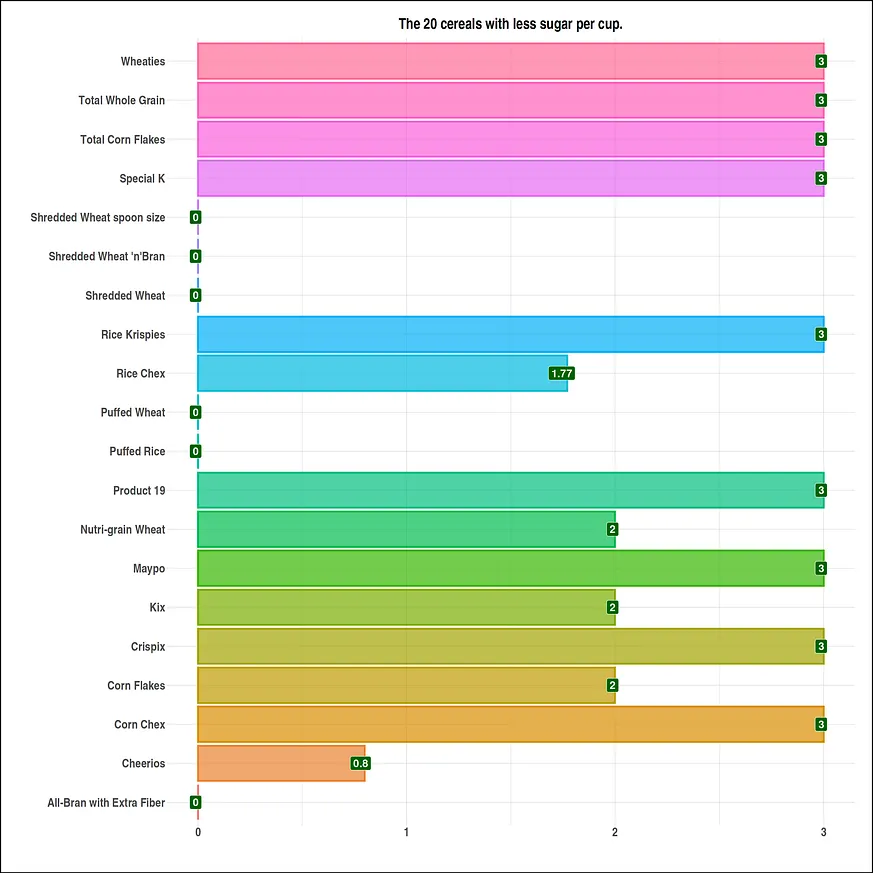
建立僅包含 Cheerios 資料的資料集
cheerios <- serving_onecup[serving_onecup$cereal == "Cheerios",] cheerios <- as.data.frame(t(cheerios[,-1])) names(cheerios)[1]<-paste("cheerios") cheerios 
建立僅包含 All-Bran 資料的資料集
allbran <- serving_onecup[serving_onecup$cereal == "All-Bran",] allbran <- as.data.frame(t(allbran[,-1])) names(allbran)[1]<-paste("AllBran") allbran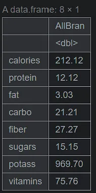
資料視覺化宣告
#visual size options(repr.plot.width = 20, repr.plot.height = 10) #Cheerios data df <- cheerios Cheerios <- ggplot(data = df, mapping = aes(x = row.names(df), y = cheerios)) + geom_segment(aes(xend=row.names(df), yend=0, color = row.names(df)), size = 2, alpha = .5) + geom_point(mapping = aes(fill = row.names(df)), size = 4, shape = 21) + coord_flip() + theme_economist() + ggtitle("Cheerios - Nutrition facts") + xlab("") + ylab("") + theme(plot.background = element_rect(fill = "#F8F8FF", color = "purple"), axis.title.x = element_text(size = 13, face = "italic"), axis.title.y = element_text(size = 13,face = "italic"), axis.text.x = element_text(size = 13, face = "bold"), axis.text.y = element_text(size = 13, face = "bold"), legend.position = "none") #All-Bran data df1 <- allbran AllBran <- ggplot(data = df1, mapping = aes(x = row.names(df1), y = AllBran)) + geom_segment(aes(xend=row.names(df1), yend=0, color = row.names(df1)), size = 2, alpha = .5) + geom_point(mapping = aes(fill = row.names(df1)), size = 4, shape = 21) + coord_flip() + theme_economist() + ggtitle("All-Bran - nutrition facts") + xlab("") + ylab("") + theme(plot.background = element_rect(fill = "#F8F8FF", color = "purple"), axis.title.x = element_text(size = 13, face = "italic"), axis.title.y = element_text(size = 13,face = "italic"), axis.text.x = element_text(size = 13, face = "bold"), axis.text.y = element_text(size = 13, face = "bold"), legend.position = "none")我們會繪製資料視覺化圖表。
plot_grid(Cheerios, Cheerios + coord_polar() , ncol = 2, nrow = 1)
plot_grid(AllBran, AllBran + coord_polar(), ncol = 2, nrow = 1)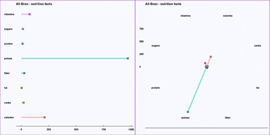
謝謝!
參考來源
全穀穀物的營養與保健功能
一、全穀的定義. 全穀是指稻米、小麥、玉米、薏. 仁等各種穀物中全部可食用的部分,. 由麩皮、胚乳和胚芽等3 部分組成。 根據歐盟2005-2010 年的健康穀物計畫.
來源: 臺中區農業改良場國民健康署也重視的全穀飲食-全穀的健康意義- 有其田
國民健康署呼籲,應該多食用保持天然型態的「原型食物」,全穀保留穀物完整型態,營養成分比精製穀類完整,營養也更豐富。有許多常吃到的穀類,也是實用全穀型 ...
來源: havefarm.com111年12月吃全穀,健康GOOD! - 營養教育專欄
穀物所去除的外層包含麩層與胚芽,其含有豐富的維生素B1、B2、維生素E和礦物質如磷、鎂、鉀等,膳食纖維的含量也是遠遠多於精製後的穀物。而其他根莖類主食如南瓜、地瓜、 ...
來源: 健康飲食運動地圖網6大類食物
全榖雜糧類 白米飯是最常被當作主食的全榖雜糧類食物,但搭配其他全榖雜糧類例如:糙米飯、全麥饅頭、甘藷、紅豆、綠豆等來獲取其他營養素(維生素B群、維生素E、礦物質及 ...
來源: 衛生福利部國民健康署穀物類- 衞生防護中心
穀物類. 營養價值. 含豐富碳水化合物; 少量維生素B1、B6; 含植物性蛋白質; 全穀物食物更含有豐富膳食纖維、礦物質如錳和鋅. 主要功用. 碳水化合物是身體的 ...
主食全谷化意義重大,專家教你怎麼吃夠全谷物
《中國居民膳食指南(2022)》建議,每天攝入谷類食物200-300克,其中全谷物和雜豆類50-150克。 “主食全谷化包含三層含義,第一層含義是'主食',它為我們機體 ...
來源: 人民网原來五穀雜糧營養與好處這麼多!但小心這些人並不適合穀物飲食。
穀物(Grain)是人類最大的食品能源之一,其中分為全穀物和精緻穀物,這兩者的營養價值可是相差甚遠。所謂「全穀物」的定義是指整顆穀物經過處理後仍然保有與原穀物比例 ...
來源: 溫室好食道均衡飲食第一步,全榖雜糧吃起來 - 福穀樂包子
加上實證營養學原則,提出適合多數台灣人的飲食建議,製訂出「每日飲食指南」,涵蓋六大類食物:全穀雜糧類、豆魚蛋肉類、乳品類、蔬菜類、水果類、油脂與堅果 ...
來源: fukurobun.com.tw
 全部
全部 康健
康健
相關討論