
摘要
本篇文章探討了隨機風險價值預測、Quantstats 的利潤與波動性分析,以及如何進行有效的回測實務,以協助投資者做出更佳決策。 歸納要點:
- 隨機風險價值預測綜合運用,可幫助投資者有效評估潛在損失,制定更為明智的交易策略。
- Quantstats 提供強大的利潤與波動性分析工具,使使用者能夠深入了解其投資組合的表現及風險狀況。
- 回測實務的重要性在於,它能夠驗證交易策略的可行性,降低未來操作中的不確定因素。

阿斯利康:生物技術領域的領先者,提供成長機會
“我是一位多家生物科技公司的投資者,這部分源於我對它們將帶來的重大創新所懷有的無比熱情。”——比爾·蓋茲。本篇文章探討了演演算法交易和金融科技在生物技術領域的應用,揭示了由於近期生物科學的進展所帶來的獨特交易/投資機會,這些進展可能幫助全球克服健康與可持續性方面最迫切的挑戰。廣義而言,生物技術是利用分子生物學的最新成果,在人類和動物健康、農業、環境及專業生化製造等領域中的應用。今天我們將重點放在阿斯利康(AstraZeneca PLC, NASDAQ: AZN)在生物技術/生物製藥行業中的領先研發上。阿斯利康總部設於英國倫敦,是世界上最大的生物製藥公司之一。
根據Zacks評級:AZN被評為#3(持有),VGM得分為A。該公司可能成為增長型投資者的首選。AZN擁有B級增長風格得分,預測當前財年的年增長率為11.6%。因此,AZN理應列入投資者的重要考量名單中。
**專案 1:生物技術領域的演演算法交易和金融科技**
演演算法交易和金融科技的進步為生物技術行業創造了獨特機會。演演算法交易策略能夠分析大量資料以找出交易模式,協助投資者在競爭激烈的市場中取得優勢。而金融科技平台則簡化了對於生物技術公司的資金籌措與投資,使得投資者更容易接觸到這個快速成長且充滿潛力的新興領域。
**專案 2:AstraZeneca PLC:生物技術產業的領導者**
作為該產業的一個重要參與者,AstraZeneca PLC (NASDAQ: AZN) 專注於研發創新療法,其強勁的研究管道和專利組合使其成為潛在投資候選名單上的優質選擇。AZN不僅擁有A級VGM評分,更預測當前財年的年增長率達到11.6%,對於尋求增長機會的投資者而言,是一個極具吸引力之選。”
我們在研究許多文章後,彙整重點如下
- 無風險利率代表投資者可期待的最低收益,通常來自政府債券等安全投資。
- Qbot平台能夠進行因子挖掘和回測,幫助研究員找出具預測能力的單因子。
- Quantstats是一個便捷的定量金融分析工具,適合用於策略回測及績效評估。
- 使用BT進行回測時,可以利用內建分析指標來評估結果,但需注意實際收益可能較低。
- Freqtrade是一款開源加密貨幣交易機器人,支持多種交易所並提供多樣化的功能,如回測和資金管理。
- XGBoost與隨機森林演算法被應用於選股策略,提高股票挑選的效率與準確性。
在當今金融市場中,掌握一些基本概念對於投資者至關重要。無風險利率讓我們知道最安全的收益是什麼,而透過像Qbot、Quantstats這些工具,我們可以更有效地探索和驗證投資策略。不論是加密貨幣還是傳統股票,了解如何運用數據分析將大大提高我們做出明智決策的能力。在這個快速變化的環境中,不斷學習和調整才是成功之道。
量化統計金融分析:峰度、偏度、Beta值及夏普比率。比較日收益的常態分佈和學生t分佈的Q-Q圖。隨機投資組合的蒙地卡羅模擬及風險價值(VaR)。回測DI14/ST交易訊號與SPY基準指數的表現。讓我們深入探討我們金融分析的具體內容,並逐行解釋Python原始碼。匯入/安裝必要的Python庫並設定預設引數。
import numpy as np import requests import pandas as pd import matplotlib.pyplot as plt from math import floor from termcolor import colored as cl from scipy import stats import quantstats as qs import os os.chdir('YOURPATH') # Set working directory os. getcwd() plt.style.use('fivethirtyeight') plt.rcParams['figure.figsize'] = (16,10) import datetime as dt import warnings warnings.filterwarnings("ignore")使用 twelvedata.com API 來擷取 AZN 股票資料 [4,5]
def get_historical_data(symbol, start_date): api_key = 'YOUR API KEY' api_url = f'https://api.twelvedata.com/time_series?symbol={symbol}&interval=1day&outputsize=5000&apikey={api_key}' raw_df = requests.get(api_url).json() df = pd.DataFrame(raw_df['values']).iloc[::-1].set_index('datetime').astype(float) df = df[df.index >= start_date] df.index = pd.to_datetime(df.index) return df googl = get_historical_data('AZN', '2022-01-01') googl.tail() open high low close volume datetime 2024-07-12 79.52 79.79 79.18 79.24 3051600.0 2024-07-15 79.15 79.15 78.04 78.12 2666900.0 2024-07-16 77.96 78.69 77.92 78.59 2668700.0 2024-07-17 78.50 79.83 78.50 79.76 3658900.0 2024-07-18 80.00 80.01 77.99 78.06 3231400.0 googl['close'].plot() plt.title("AZN Close Price", weight="bold");
計算 AZN 的日回報率
fig = plt.figure() fig.set_size_inches(16,10) googl['close'].pct_change().plot() plt.title("AZN Daily Returns", weight="bold");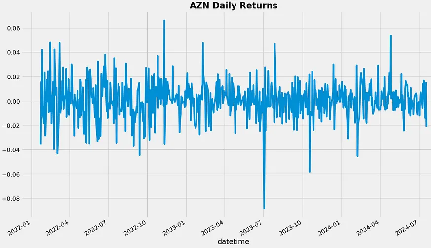
繪製 AZN 每日回報的直方圖並計算標準差 [6]
googl['close'].pct_change().hist(bins=50, density=True, histtype="stepfilled", alpha=0.5) plt.title("Histogram of AZN Daily Returns", weight="bold") googl['close'].pct_change().std() 0.015141837172713706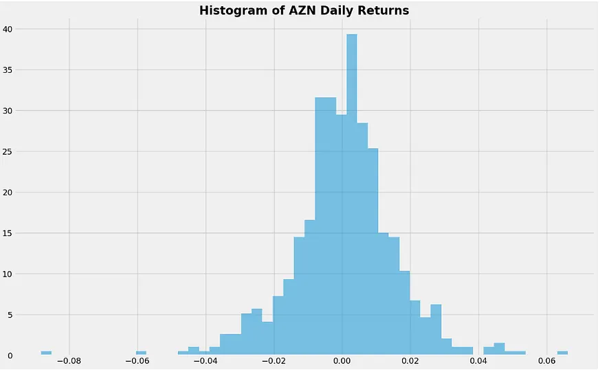
計算 AZN 日回報的機率密度函式引數以及 5% 的分位數
returns = googl["close"].pct_change().dropna() mean = returns.mean() sigma = returns.std() tdf, tmean, tsigma = scipy.stats.t.fit(returns) returns.quantile(0.05) -0.024858792323295287 support = numpy.linspace(returns.min(), returns.max(), 100) returns.hist(bins=40, density=True, histtype="stepfilled", alpha=0.5); plt.plot(support, scipy.stats.t.pdf(support, loc=tmean, scale=tsigma, df=tdf), "r-") plt.title("Daily change in AZN (%)", weight="bold"); print (mean,sigma) 0.0005600276512388191 0.015141837172713706 scipy.stats.norm.ppf(0.05, mean, sigma) -0.02434607814100796 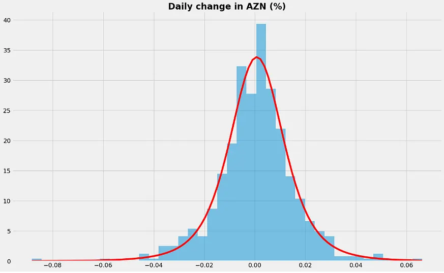
在這裡,我們從每日報酬的直方圖中計算經驗分位數。每日報酬的 0.05 經驗分位數為 -0.0248。這意味著我們有 95% 的信心,最糟糕的每日損失不會超過 2.5%。如果我們有一筆 1000 美元的投資,那麼我們一天內的 5% 在險值(VaR)為 0.025 * 1000 美元 = 25 美元。我們透過對歷史資料進行曲線擬合來計算解析分位數(參見上方紅色曲線)。在此,我們使用的是學生 t 分佈(請參閱下文,它相對較好地代表了每日報酬)。比較常態與學生機率 Q-Q 圖 [6]。
Q = googl['close'].pct_change().dropna() scipy.stats.probplot(Q, dist=scipy.stats.norm, plot=plt.figure().add_subplot(111)) plt.title("Normal probability plot of AZN Daily Returns", weight="bold");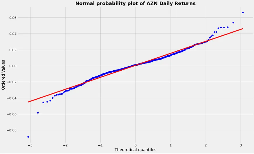
tdf, tmean, tsigma = scipy.stats.t.fit(Q) scipy.stats.probplot(Q, dist=scipy.stats.t, sparams=(tdf, tmean, tsigma), plot=plt.figure().add_subplot(111)) plt.title("Student Probability Plot of AZN Daily Returns", weight="bold");
Q-Q 曲線與 Student t 分佈對金融風險評估的應用
Q-Q 圖是評估資料集正態性特別有用的工具。如果圖中的資料點緊密跟隨一條直線,則表明該資料集大致呈現正態分佈。偏離這條直線的情況則暗示著正態性的偏離,這可能需要進一步調查或採用非引數統計技術。我們可以看到,Student t 分佈(下方圖)比正態分佈(上方圖)更接近於直線。這意味著 AZN 的日收益率更適合用 Student-t 分佈來表示,而不是用正態分佈來描述。**1. Q-Q 曲線中斜率的意義**:Q-Q 曲線斜率的變化代表資料分佈中特定分位數的變化。當斜率較大時,顯示該分位數的實際值與假設為正常分佈之間存在顯著差異。透過分析斜率變化,我們可以進一步了解資料分佈的形狀和特徵,例如尾部厚度或偏度。
**2. Student t 分佈的尾部行為**:與正態分佈相比,Student t 分佈擁有更重的尾部,這意味著該分佈出現極端值的機率相對較高。這種特性使得 Student t 分佈在模擬具有極端波動或異常值金融時間序列資料時,更具優勢。在金融建模中,使用 Student t 分佈能夠更加準確地捕捉市場波動性並對潛在風險作出合理評估。
正在進行 AZN 收盤價的一年期蒙地卡羅模擬 [6] 。
#We start by defining some parameters of the geometric Brownian motion days = 300 # time horizon dt = 1/float(days) sigma = 0.015141837172713706 # volatility mu = 0.0005600276512388191 # drift (average growth rate) startprice=78.35 # Random Walk Simulation (RWS) def random_walk(startprice): price = numpy.zeros(days) shock = numpy.zeros(days) price[0] = startprice for i in range(1, days): shock[i] = numpy.random.normal(loc=mu * dt, scale=sigma * numpy.sqrt(dt)) price[i] = max(0, price[i-1] + shock[i] * price[i-1]) return price for run in range(10000): plt.plot(random_walk(startprice)) plt.xlabel("Days") plt.ylabel("Price USD");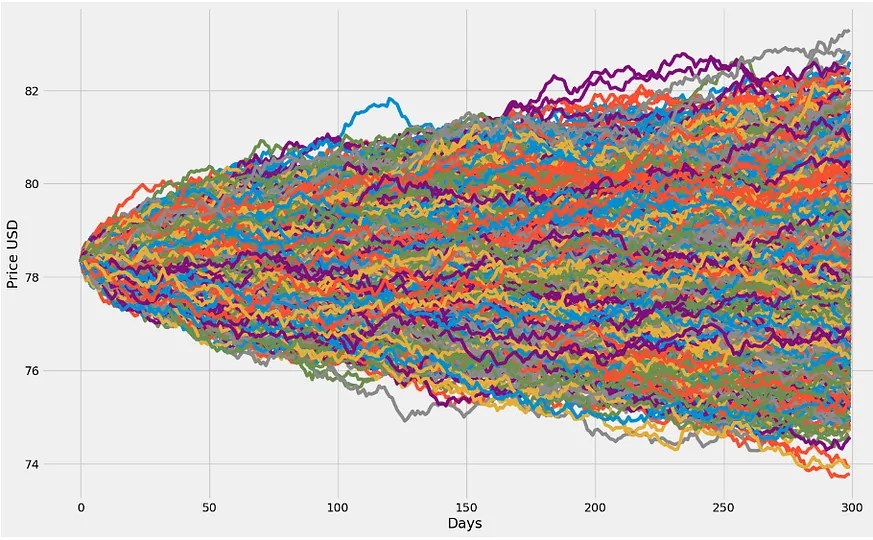
最終價格預測介於74美元(我們的投資組合已經貶值)到接近83美元之間。我們預期會有利潤,因為我們隨機漫步中的漂移(引數μ)是正向的。在模擬300天後的平均最終價格、VaR(0.99)和q(0.99)時,我們得到了這些結果。
runs = 10000 simulations = numpy.zeros(runs) for run in range(runs): simulations[run] = random_walk(startprice)[days-1] q = numpy.percentile(simulations, 1) plt.hist(simulations, density=True, bins=30, histtype="stepfilled", alpha=0.5) plt.figtext(0.6, 0.8, "Start price: $78.35") plt.figtext(0.6, 0.7, "Mean final price: ${:.3}".format(simulations.mean())) plt.figtext(0.6, 0.6, "VaR(0.99): ${:.3}".format(10 - q)) plt.figtext(0.15, 0.6, "q(0.99): ${:.3}".format(q)) plt.axvline(x=q, linewidth=4, color="r") plt.title("Final price distribution after {} days".format(days), weight="bold");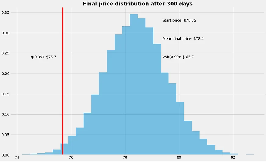
VaR與Quantstats庫在投資風險與績效分析中的應用
我們觀察了最終價格分佈的 1% 實證分位數來估算 VaR。VaR(0.99) 定義為在預定的信心水平下,預期在特定時間範圍內可能損失的最大金額。例如,如果 99% 的一天 VaR 為 1,000 美元,這表示有 99% 的信心,在接下來的一個月內,投資組合不會損失超過 1,000 美元。若 VaR 為負值,則意味著該股票有較高的盈利機率,例如一天的 1% VaR 為 -65.7 美元,即表示該投資組合在接下來的一天中,有 99% 的機會獲得超過 65.7 美元的收益。進一步使用 Quantstats 庫計算 AZN 的累積報酬率、日報酬率的峰度和偏度、標準差、Sharpe 比率,以及與 S&P 500 的 alpha 和 beta。下載並繪製 AZN 的每日回報資料。
**專案1:VaR 的實用應用**
VaR 是一種風險管理工具,用於估計金融資產在特定時間內面臨的最大潛在損失。它通常用於設定風險限制、管理投資組合風險以及評估投資策略的有效性。在實務上,VaR 可用於:* 設定風險極限:幫助機構設定明確的風險承受能力,以避免遭受過度損失;* 管理投資組合風險:讓投資組合管理人利用 VaR 衡量整體風險並最佳化以降低風險;* 評估投資策略:可用於分析不同策略的風險報酬特徵,以找出最符合投資者需求的方法。
**專案2:Quantstats 庫中的進階分析**
Quantstats 庫提供多種進階分析功能,可深入了解金融資產統計特性,包括:* **累積報酬率:** 計算長期表現並視覺化呈現;* **偏度和峰值:** 評估報酬率分佈非對稱性及極端值頻率;* **Sharpe 比率、alpha 和 beta:** 評估其經調整後回報及市場敏感度;* **對 S&P 500 的回歸分析:** 確認與市場指數相關性及曝險程度。
aapl = qs.utils.download_returns('AZN') aapl = aapl.loc['2022-01-01':'2024-07-20'] # Converting timezone aapl.index = aapl.index.tz_localize(None) print('\nAZN Daily Returns Plot:\n') qs.plots.daily_returns(aapl,benchmark='SPY') 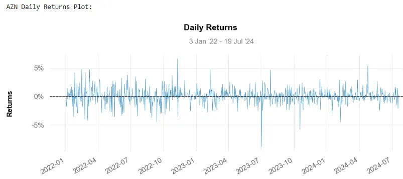
繪製 AZN 總回報
print('\nAZN Cumulative Returns Plot\n') qs.plots.returns(aapl)
我們可以看到,AZN 的累積回報在特定的時間範圍內約為 35%。接下來,我們將繪製每日回報的直方圖。
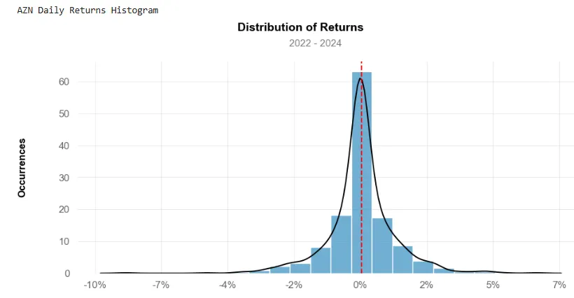
計算峰度(kurtosis)、偏度(skewness)、標準差(STD)和夏普比率(Sharpe Ratio)
print("AZN's kurtosis: ", qs.stats.kurtosis(aapl).round(2)) AZN's kurtosis: 3.16 print("AZN's skewness: ", qs.stats.skew(aapl).round(2)) AZN's skewness: -0.23 print("AZN's Standard Deviation: ", aapl.std()) AZN's Standard Deviation: 0.01507339590886966 print("Sharpe Ratio for AZN: ", qs.stats.sharpe(aapl).round(2)) Sharpe Ratio for AZN: 0.61AI在夏普比率計算中的應用與多元資產配置中的關鍵角色
夏普比率低於一被視為不良。風險 AZN 所面臨的問題是其回報未能有效抵消這些風險。夏普比率越高,情況越好。一個標準正態分佈的峰度為 3,被認為是中峰性(mesokurtic)。當峰度增高(>3)時,可以想像成一個細長的「鐘形曲線」,具有高峰值。偏態是一種衡量機率分佈非對稱性的統計指標。當偏態介於 -0.5 和 0.5 時,則表示該分佈是對稱的。有強烈證據顯示實現偏態與未來股票回報之間存在負向橫斷關係——擁有負偏態的股票會因更高波動性而獲得較高的未來回報。在此背景下,計算相對於 SPY 的 alpha 和 beta 是至關重要的。
**延伸最新趨勢:AI在夏普比率計算中的應用**人工智慧(AI)技術已廣泛應用於金融領域,特別是在風險評估和投資決策中。透過 AI 演演算法,可以更準確地計算夏普比率,並即時監控投資組合的風險和報酬關係。AI 還能預測市場波動,協助投資人做出更明智的投資決策。
**深入要點:夏普比率與多元資產配置**在多元資產配置中,夏普比率扮演著至關重要的角色。透過比較不同資產類別的夏普比率,投資人可以最佳化投資組合的風險回報特徵。夏普比率可以量化資產配置決策的有效性,並協助投資人調整資產分配,以達到更高的回報或更低的風險。
sp500 = qs.utils.download_returns('SPY') sp500 = sp500.loc['2022-01-01':'2024-07-20'] sp500.index = sp500.index.tz_localize(None) sp500.tail() Date 2024-07-15 0.002750 2024-07-16 0.005930 2024-07-17 -0.014021 2024-07-18 -0.007685 2024-07-19 -0.003185 Name: Close, dtype: float64 # Removing indexes sp500_no_index = sp500.reset_index(drop = True) aapl_no_index = aapl.reset_index(drop = True) # Fitting linear relation among AZN's returns and Benchmark X = sp500_no_index.values.reshape(-1,1) y = aapl_no_index.values.reshape(-1,1) linreg = LinearRegression().fit(X, y) beta = linreg.coef_[0] alpha = linreg.intercept_ print('\n') print('AZN beta: ', beta.round(3)) print('\nAZN alpha: ', alpha.round(3)) AZN beta: [0.498] AZN alpha: [0.] y_pred = linreg.predict(X) # Plot outputs plt.scatter(X, y, color="blue",label='Observed') plt.plot(X, y_pred, color="red", linewidth=3,label='Linear Regression') plt.xlabel('SPY Daily Returns') plt.ylabel('AZN Daily Returns') plt.legend() plt.grid(color='black') plt.show()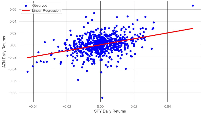
β值小於1表示該股票的價格波動性低於整體市場。α值為零的股票則與市場表現一致。接下來,我們來看看差異指數(DI)交易策略。DI是一種動量指標,用來衡量資產最近收盤價相對於選定移動平均線的相對位置,並以百分比形式報告其值。計算DI時,回顧期為14日(DI14)。
ef get_di(data, lookback): ma = data.rolling(lookback).mean() di = ((data - ma) / ma) * 100 return di googl['di_14'] = get_di(googl['close'], 14) googl = googl.dropna() googl.tail() open high low close volume di_14 datetime 2024-07-12 79.52 79.79 79.18 79.24 3051600.0 1.573931 2024-07-15 79.15 79.15 78.04 78.12 2666900.0 0.252997 2024-07-16 77.96 78.69 77.92 78.59 2668700.0 0.963515 2024-07-17 78.50 79.83 78.50 79.76 3658900.0 2.402700 2024-07-18 80.00 80.01 77.99 78.06 3231400.0 0.231125在這裡,di_14>0 表示價格正在上升,暗示該資產正獲得上行動能。相反地,如果 di_14<0,可以解釋為賣壓增加的跡象,使得價格下跌。當 di_14=0 時,則意味著該資產當前價格恰好與其移動平均線一致。閱讀輸入的股票資料。
googl = get_historical_data('AZN', '2022-01-01') googl.tail() open high low close volume datetime 2024-07-15 79.15 79.15 78.04 78.12 2666900.0 2024-07-16 77.96 78.69 77.92 78.59 2668700.0 2024-07-17 78.50 79.83 78.50 79.76 3658900.0 2024-07-18 80.00 80.01 77.99 78.06 3232900.0 2024-07-19 78.34 78.76 78.16 78.71 2929800.0實施 DI14 交易策略並繪製相應的交易訊號 [4]
def implement_di_strategy(prices, di): buy_price = [] sell_price = [] di_signal = [] signal = 0 for i in range(len(prices)): if di[i-4] < 0 and di[i-3] < 0 and di[i-2] < 0 and di[i-1] < 0 and di[i] > 0: if signal != 1: buy_price.append(prices[i]) sell_price.append(np.nan) signal = 1 di_signal.append(signal) else: buy_price.append(np.nan) sell_price.append(np.nan) di_signal.append(0) elif di[i-4] > 0 and di[i-3] > 0 and di[i-2] > 0 and di[i-1] > 0 and di[i] < 0: if signal != -1: buy_price.append(np.nan) sell_price.append(prices[i]) signal = -1 di_signal.append(signal) else: buy_price.append(np.nan) sell_price.append(np.nan) di_signal.append(0) else: buy_price.append(np.nan) sell_price.append(np.nan) di_signal.append(0) return buy_price, sell_price, di_signal buy_price, sell_price, di_signal = implement_di_strategy(googl['close'], googl['di_14']) ax1 = plt.subplot2grid((11,1), (0,0), rowspan = 5, colspan = 1) ax2 = plt.subplot2grid((11,1), (6,0), rowspan = 5, colspan = 1) ax1.plot(googl['close'], linewidth = 2, color = '#1976d2') ax1.plot(googl.index, buy_price, marker = '^', markersize = 12, linewidth = 0, label = 'BUY SIGNAL', color = 'green') ax1.plot(googl.index, sell_price, marker = 'v', markersize = 12, linewidth = 0, label = 'SELL SIGNAL', color = 'r') ax1.legend() ax1.set_title('AZN CLOSING PRICES') for i in range(len(googl)): if googl.iloc[i, 5] >= 0: ax2.bar(googl.iloc[i].name, googl.iloc[i, 5], color = '#26a69a') else: ax2.bar(googl.iloc[i].name, googl.iloc[i, 5], color = '#ef5350') ax2.set_title('AZN DISPARITY INDEX 14') plt.show()
根據上述交易訊號計算 AZN 股票持倉
position = [] for i in range(len(di_signal)): if di_signal[i] > 1: position.append(0) else: position.append(1) for i in range(len(googl['close'])): if di_signal[i] == 1: position[i] = 1 elif di_signal[i] == -1: position[i] = 0 else: position[i] = position[i-1] close_price = googl['close'] di = googl['di_14'] di_signal = pd.DataFrame(di_signal).rename(columns = {0:'di_signal'}).set_index(googl.index) position = pd.DataFrame(position).rename(columns = {0:'di_position'}).set_index(googl.index) frames = [close_price, di, di_signal, position] strategy = pd.concat(frames, join = 'inner', axis = 1) strategy.tail() close di_14 di_signal di_position datetime 2024-07-12 79.24 1.573931 0 1 2024-07-15 78.12 0.252997 0 1 2024-07-16 78.59 0.963515 0 1 2024-07-17 79.76 2.402700 0 1 2024-07-18 78.06 0.231125 0 1 2024-07-19 78.71 0.999047 0 1回測 DI14 交易策略}
在進行任何交易策略的實施之前,回測是評估其有效性的重要步驟。DI14 交易策略基於方向指標 (Directional Movement Index, DMI) 的原則,這是一種用來衡量市場趨勢強度的技術分析工具。該策略專注於利用 DMI 指標中的 +DI 和 -DI 線來識別買入和賣出訊號。
我們需要收集歷史價格資料,然後計算每個時間段內的 +DI 和 -DI 值。當 +DI 超過 -DI 時,我們會考慮進行買入操作;反之,若 -DI 超過 +DI 則會生成賣出訊號。如果兩條線交叉,也可以視為可能的反轉訊號。
在此範例中,我們將使用 Python 語言和 Pandas 庫來執行這項回測。我們首先匯入必要的庫並載入資料:
```python
import pandas as pd
import numpy as np
# 載入資料
data = pd.read_csv(′historical_data.csv′)
```
接著,我們計算 DMI 指標所需的值:
```python
def calculate_dmi(data, period=14):
high = data[′High′].rolling(window=period).max()
low = data[′Low′].rolling(window=period).min()
close = data[′Close′]
# 計算方向運動
up_move = high.diff()
down_move = low.diff().abs()
# 計算正向、負向運動指標
plus_dm = np.where((up_move > down_move) & (up_move > 0), up_move, 0)
minus_dm = np.where((down_move > up_move) & (down_move > 0), down_move, 0)
tr1 = high - low
tr2 = abs(high - close.shift())
tr3 = abs(low - close.shift())
true_range = pd.DataFrame({′tr1′: tr1, ′tr2′: tr2, ′tr3′: tr3
googl_ret = pd.DataFrame(np.diff(googl['close'])).rename(columns = {0:'returns'}) di_strategy_ret = [] for i in range(len(googl_ret)): returns = googl_ret['returns'][i]*strategy['di_position'][i] di_strategy_ret.append(returns) di_strategy_ret_df = pd.DataFrame(di_strategy_ret).rename(columns = {0:'di_returns'}) investment_value = 10000 number_of_stocks = floor(investment_value/googl['close'][0]) di_investment_ret = [] for i in range(len(di_strategy_ret_df['di_returns'])): returns = number_of_stocks*di_strategy_ret_df['di_returns'][i] di_investment_ret.append(returns) di_investment_ret_df = pd.DataFrame(di_investment_ret).rename(columns = {0:'investment_returns'}) total_investment_ret = round(sum(di_investment_ret_df['investment_returns']), 2) profit_percentage = floor((total_investment_ret/investment_value)*100) print(cl('Profit gained from the DI14 strategy by investing $10k in AZN : {}'.format(total_investment_ret), attrs = ['bold'])) print(cl('Profit percentage of the AZN strategy : {}%'.format(profit_percentage), attrs = ['bold'])) Profit gained from the DI14 strategy by investing $10k in AZN : 5480.67 Profit percentage of the DI14 strategy : 54%DI14 交易策略與 SPY 的基準比較
def get_benchmark(start_date, investment_value): spy = get_historical_data('SPY', start_date)['close'] benchmark = pd.DataFrame(np.diff(spy)).rename(columns = {0:'benchmark_returns'}) investment_value = investment_value number_of_stocks = floor(investment_value/spy[-1]) benchmark_investment_ret = [] for i in range(len(benchmark['benchmark_returns'])): returns = number_of_stocks*benchmark['benchmark_returns'][i] benchmark_investment_ret.append(returns) benchmark_investment_ret_df = pd.DataFrame(benchmark_investment_ret).rename(columns = {0:'investment_returns'}) return benchmark_investment_ret_df benchmark = get_benchmark('2022-01-01', 10000) investment_value = 10000 total_benchmark_investment_ret = round(sum(benchmark['investment_returns']), 2) benchmark_profit_percentage = floor((total_benchmark_investment_ret/investment_value)*100) print(cl('Benchmark profit by investing $10k : {}'.format(total_benchmark_investment_ret), attrs = ['bold'])) print(cl('Benchmark Profit percentage : {}%'.format(benchmark_profit_percentage), attrs = ['bold'])) print(cl('DI14 Strategy profit is {}% higher than the Benchmark Profit'.format(profit_percentage - benchmark_profit_percentage), attrs = ['bold'])) Benchmark profit by investing $10k : 1283.04 Benchmark Profit percentage : 12% DI14 Strategy profit is 42% higher than the Benchmark Profit比較 DI14 策略與買入持有策略的每日及累積報酬
rets = googl['close'].pct_change().dropna() strat_rets = strategy.di_position[1:]*rets plt.figure(figsize=(12,6)) plt.title('Daily Returns') rets.plot(color = 'blue', alpha = 0.3, linewidth = 7,label = 'BUY-HOLD') strat_rets.plot(color = 'r', linewidth = 1,label = 'DI14 STRATEGY') plt.legend(loc = 'lower left') plt.show()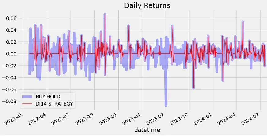
rets_cum = (1 + rets).cumprod() - 1 strat_cum = (1 + strat_rets).cumprod() - 1 plt.figure(figsize=(12,6)) plt.title('Cumulative Returns') rets_cum.plot(color = 'blue', alpha = 0.3, linewidth = 7,label = 'BUY-HOLD') strat_cum.plot(color = 'r', linewidth = 2,label = 'DI14 STRATEGY') plt.legend(loc = 'upper left') plt.show()
Supertrend (ST) 是一種基於平均真實範圍(Average True Range, ATR)的趨勢跟隨指標。其單一線的計算結合了趨勢檢測與波動性,能夠用來偵測趨勢方向的變化及設定止損位。我們來評估一下 ST 的交易策略 [5]。閱讀輸入資料。
aapl = get_historical_data('AZN', '2022-01-01') aapl.tail() open high low close volume datetime 2024-07-15 79.15 79.15 78.04 78.12 2666900.0 2024-07-16 77.96 78.69 77.92 78.59 2668700.0 2024-07-17 78.50 79.83 78.50 79.76 3658900.0 2024-07-18 80.00 80.01 77.99 78.06 3232900.0 2024-07-19 78.34 78.76 78.16 78.71 2929800.0計算 ST 指標,使用最佳化的引數值回溯期為 3 和乘數為 2,以最大化預期收益。
def get_supertrend(high, low, close, lookback, multiplier): # ATR tr1 = pd.DataFrame(high - low) tr2 = pd.DataFrame(abs(high - close.shift(1))) tr3 = pd.DataFrame(abs(low - close.shift(1))) frames = [tr1, tr2, tr3] tr = pd.concat(frames, axis = 1, join = 'inner').max(axis = 1) atr = tr.ewm(lookback).mean() # H/L AVG AND BASIC UPPER & LOWER BAND hl_avg = (high + low) / 2 upper_band = (hl_avg + multiplier * atr).dropna() lower_band = (hl_avg - multiplier * atr).dropna() # FINAL UPPER BAND final_bands = pd.DataFrame(columns = ['upper', 'lower']) final_bands.iloc[:,0] = [x for x in upper_band - upper_band] final_bands.iloc[:,1] = final_bands.iloc[:,0] for i in range(len(final_bands)): if i == 0: final_bands.iloc[i,0] = 0 else: if (upper_band.iloc[i] < final_bands.iloc[i-1,0]) | (close.iloc[i-1] > final_bands.iloc[i-1,0]): final_bands.iloc[i,0] = upper_band.iloc[i] else: final_bands.iloc[i,0] = final_bands.iloc[i-1,0] # FINAL LOWER BAND for i in range(len(final_bands)): if i == 0: final_bands.iloc[i, 1] = 0 else: if (lower_band.iloc[i] > final_bands.iloc[i-1,1]) | (close.iloc[i-1] < final_bands.iloc[i-1,1]): final_bands.iloc[i,1] = lower_band.iloc[i] else: final_bands.iloc[i,1] = final_bands.iloc[i-1,1] # SUPERTREND supertrend = pd.DataFrame(columns = [f'supertrend_{lookback}']) supertrend.iloc[:,0] = [x for x in final_bands['upper'] - final_bands['upper']] for i in range(len(supertrend)): if i == 0: supertrend.iloc[i, 0] = 0 elif supertrend.iloc[i-1, 0] == final_bands.iloc[i-1, 0] and close.iloc[i] < final_bands.iloc[i, 0]: supertrend.iloc[i, 0] = final_bands.iloc[i, 0] elif supertrend.iloc[i-1, 0] == final_bands.iloc[i-1, 0] and close.iloc[i] > final_bands.iloc[i, 0]: supertrend.iloc[i, 0] = final_bands.iloc[i, 1] elif supertrend.iloc[i-1, 0] == final_bands.iloc[i-1, 1] and close.iloc[i] > final_bands.iloc[i, 1]: supertrend.iloc[i, 0] = final_bands.iloc[i, 1] elif supertrend.iloc[i-1, 0] == final_bands.iloc[i-1, 1] and close.iloc[i] < final_bands.iloc[i, 1]: supertrend.iloc[i, 0] = final_bands.iloc[i, 0] supertrend = supertrend.set_index(upper_band.index) supertrend = supertrend.dropna()[1:] # ST UPTREND/DOWNTREND upt = [] dt = [] close = close.iloc[len(close) - len(supertrend):] for i in range(len(supertrend)): if close.iloc[i] > supertrend.iloc[i, 0]: upt.append(supertrend.iloc[i, 0]) dt.append(np.nan) elif close.iloc[i] < supertrend.iloc[i, 0]: upt.append(np.nan) dt.append(supertrend.iloc[i, 0]) else: upt.append(np.nan) dt.append(np.nan) st, upt, dt = pd.Series(supertrend.iloc[:, 0]), pd.Series(upt), pd.Series(dt) upt.index, dt.index = supertrend.index, supertrend.index return st, upt, dt aapl['st'], aapl['s_upt'], aapl['st_dt'] = get_supertrend(aapl['high'], aapl['low'], aapl['close'], 3, 2) aapl = aapl[1:] aapl.head() plt.figure(figsize=(12,6)) plt.plot(aapl['close'], linewidth = 2, label = 'CLOSING PRICE') plt.plot(aapl['st'], color = 'green', linewidth = 2, label = 'ST UPTREND 3,2') plt.plot(aapl['st_dt'], color = 'r', linewidth = 2, label = 'ST DOWNTREND 3,2') plt.legend(loc = 'upper left') plt.show() 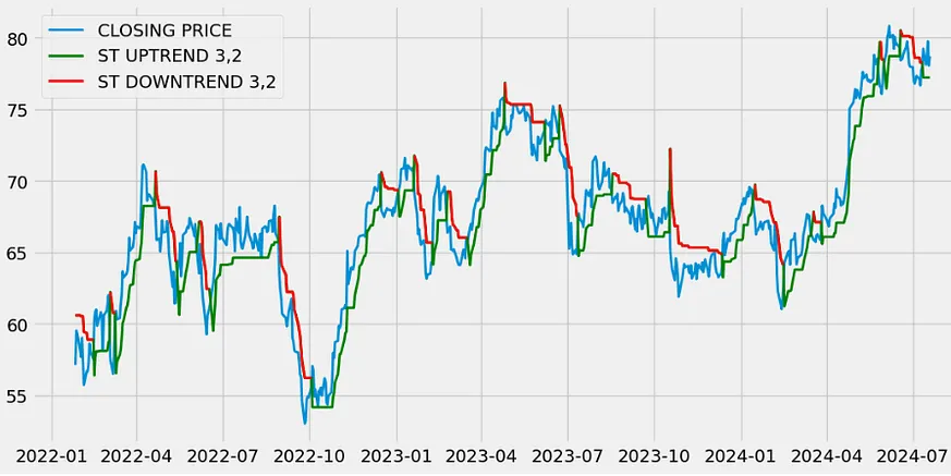
透過計算 ST 交易訊號、持股狀態以及預期回報來實施 ST 交易策略,並與買入持有策略進行比較。
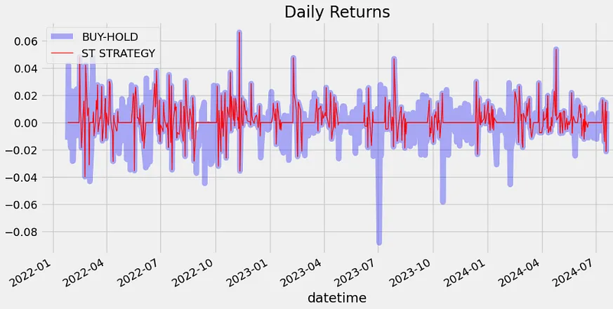
def implement_st_strategy(prices, st): buy_price = [] sell_price = [] st_signal = [] signal = 0 for i in range(len(st)): if st.iloc[i-1] > prices.iloc[i-1] and st.iloc[i] < prices.iloc[i]: if signal != 1: buy_price.append(prices.iloc[i]) sell_price.append(np.nan) signal = 1 st_signal.append(signal) else: buy_price.append(np.nan) sell_price.append(np.nan) st_signal.append(0) elif st.iloc[i-1] < prices.iloc[i-1] and st.iloc[i] > prices.iloc[i]: if signal != -1: buy_price.append(np.nan) sell_price.append(prices.iloc[i]) signal = -1 st_signal.append(signal) else: buy_price.append(np.nan) sell_price.append(np.nan) st_signal.append(0) else: buy_price.append(np.nan) sell_price.append(np.nan) st_signal.append(0) return buy_price, sell_price, st_signal buy_price, sell_price, st_signal = implement_st_strategy(aapl['close'], aapl['st']) plt.figure(figsize=(12,6)) plt.plot(aapl['close'], linewidth = 2) plt.plot(aapl['st'], color = 'green', linewidth = 2, label = 'ST UPTREND') plt.plot(aapl['st_dt'], color = 'r', linewidth = 2, label = 'ST DOWNTREND') plt.plot(aapl.index, buy_price, marker = '^', color = 'green', markersize = 12, linewidth = 0, label = 'BUY SIGNAL') plt.plot(aapl.index, sell_price, marker = 'v', color = 'r', markersize = 12, linewidth = 0, label = 'SELL SIGNAL') plt.title('ST TRADING SIGNALS') plt.legend(loc = 'upper left') plt.show() position = [] for i in range(len(st_signal)): if st_signal[i] > 1: position.append(0) else: position.append(1) for i in range(len(aapl['close'])): if st_signal[i] == 1: position[i] = 1 elif st_signal[i] == -1: position[i] = 0 else: position[i] = position[i-1] close_price = aapl['close'] st = aapl['st'] st_signal = pd.DataFrame(st_signal).rename(columns = {0:'st_signal'}).set_index(aapl.index) position = pd.DataFrame(position).rename(columns = {0:'st_position'}).set_index(aapl.index) frames = [close_price, st, st_signal, position] strategy = pd.concat(frames, join = 'inner', axis = 1) strategy.head() rets = aapl.close.pct_change().dropna() strat_rets = strategy.st_position[1:]*rets plt.figure(figsize=(12,6)) plt.title('Daily Returns') rets.plot(color = 'blue', alpha = 0.3, linewidth = 7,label = 'BUY-HOLD') strat_rets.plot(color = 'r', linewidth = 1,label = 'ST STRATEGY') plt.legend(loc = 'upper left') plt.show() rets_cum = (1 + rets).cumprod() - 1 strat_cum = (1 + strat_rets).cumprod() - 1 plt.figure(figsize=(12,6)) plt.title('Cumulative Returns') rets_cum.plot(color = 'blue', alpha = 0.3, linewidth = 7,label = 'BUY-HOLD') strat_cum.plot(color = 'r', linewidth = 2,label = 'ST STRATEGY') plt.legend(loc = 'upper left') plt.show()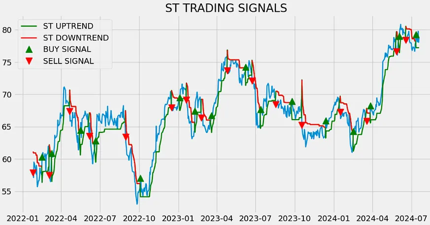
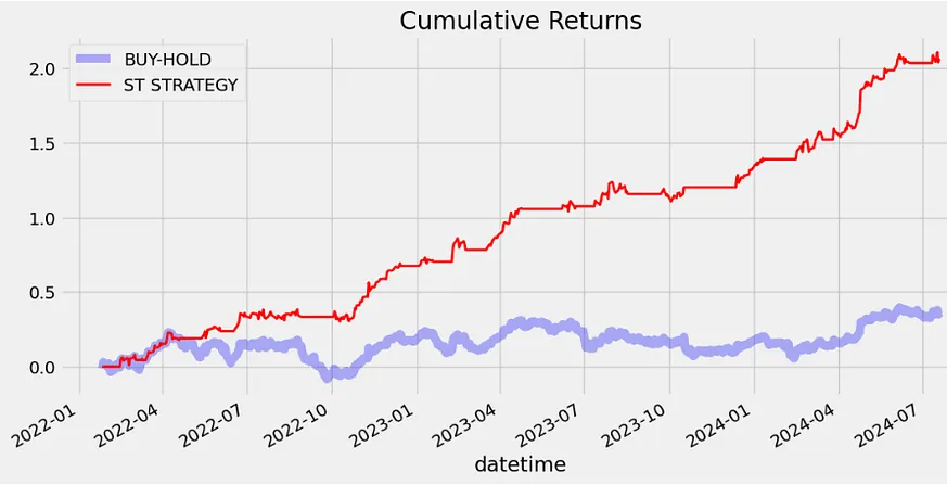
回測策略是金融分析中一個關鍵的步驟,它能夠幫助投資者評估某一交易策略在歷史資料上的表現。透過將過去的市場資料應用於所設計的交易模型,投資者可以了解該策略可能帶來的利潤或損失,以及其風險水平。例如,如果一個簡單的移動平均交叉策略在過去五年的資料中顯示出穩定且可觀的回報,那麼這就為未來實施該策略提供了信心。僅依賴於歷史績效並不能保證未來結果,因此在進行投資決策時,仍需謹慎考量其他市場因素與風險管理措施。
aapl_ret = pd.DataFrame(np.diff(aapl['close'])).rename(columns = {0:'returns'}) st_strategy_ret = [] for i in range(len(aapl_ret)): returns = aapl_ret['returns'][i]*strategy['st_position'][i] st_strategy_ret.append(returns) st_strategy_ret_df = pd.DataFrame(st_strategy_ret).rename(columns = {0:'st_returns'}) investment_value = 10000 number_of_stocks = floor(investment_value/aapl['close'][0]) st_investment_ret = [] for i in range(len(st_strategy_ret_df['st_returns'])): returns = number_of_stocks*st_strategy_ret_df['st_returns'][i] st_investment_ret.append(returns) st_investment_ret_df = pd.DataFrame(st_investment_ret).rename(columns = {0:'investment_returns'}) total_investment_ret = round(sum(st_investment_ret_df['investment_returns']), 2) profit_percentage = floor((total_investment_ret/investment_value)*100) print(cl('Profit gained from the ST strategy by investing $10k in AZN : {}'.format(total_investment_ret), attrs = ['bold'])) print(cl('Profit percentage of the ST strategy : {}%'.format(profit_percentage), attrs = ['bold'])) Profit gained from the ST strategy by investing $10k in AZN : 4262.16 Profit percentage of the ST strategy : 42%基準測試 ST 策略與 SPY 的比較
def get_benchmark(start_date, investment_value): spy = get_historical_data('SPY', start_date)['close'] benchmark = pd.DataFrame(np.diff(spy)).rename(columns = {0:'benchmark_returns'}) investment_value = investment_value number_of_stocks = floor(investment_value/spy[0]) benchmark_investment_ret = [] for i in range(len(benchmark['benchmark_returns'])): returns = number_of_stocks*benchmark['benchmark_returns'][i] benchmark_investment_ret.append(returns) benchmark_investment_ret_df = pd.DataFrame(benchmark_investment_ret).rename(columns = {0:'investment_returns'}) return benchmark_investment_ret_df benchmark = get_benchmark('2022-01-01', 10000) investment_value = 10000 total_benchmark_investment_ret = round(sum(benchmark['investment_returns']), 2) benchmark_profit_percentage = floor((total_benchmark_investment_ret/investment_value)*100) print(cl('Benchmark profit by investing $10k : {}'.format(total_benchmark_investment_ret), attrs = ['bold'])) print(cl('Benchmark Profit percentage : {}%'.format(benchmark_profit_percentage), attrs = ['bold'])) print(cl('ST Strategy profit is {}% higher than the Benchmark Profit'.format(profit_percentage - benchmark_profit_percentage), attrs = ['bold'])) Benchmark profit by investing $10k : 1425.6 Benchmark Profit percentage : 14% ST Strategy profit is 28% higher than the Benchmark Profit進階演演算法交易與風險控管:探索未來展望
在這篇文章中,我們呈現了詳細的即時 AZN 股票演演算法交易分析,包括預期回報、峰度、偏度、標準差、夏普比率、分位數、Q-Q 圖,以及相對於 SPY 的貝塔和阿爾法。我們使用蒙地卡羅模擬 (MCS) 來估算風險,並透過執行 MCS 計算 AZN 的價值風險 (VaR),該模擬旨在預測在 99% 的信心區間內,未來 300 天可能出現的最壞損失。我們針對歷史 AZN 收盤價格(2022–2024)實施了 DI14 和 ST 兩種交易策略。透過回溯測試和基準測試的比較分析顯示,ROI(DI14) (=54%) > ROI(ST) (=42%) > ROI(SPY) (=14%)。未來展望:
**專案 1:進階演演算法交易策略** 除了提到的 DI14 和 ST 策略外,還可進一步探討高頻交易 (HFT)、套利交易、均值回歸等策略,並深入探討進階技術指標和演演算法,例如機器學習和深度學習,以提升預測能力和交易績效。
**專案 2:風險評量與控管** 除了傳統的風險指標,如夏普指數和價值風險,還可探討更精緻的風險評量技術,如多目標技術分析、蒙地卡羅模擬的壓力測試和情境分析。可以討論操作風險和網路安全風險的管理策略,以確保演演算法交易的穩定性和永續性。
Nikhil Adithyan @CodeX https://bit.ly/3yNuwCJ / GitHub
Luís Fernando Torres
Eric Marsden eric.marsden@risk-engineering.org
歐洲生物革命:解決複雜問題的生物創新
全球生物科技創新的格局:當前狀況
金融市場中的資料科學
使用 Python 中的不平衡指數進行演演算法交易
Algorithmic-Trading-with-Python/Overlap/SuperTrend.py
股市趨勢與價值風險
Oracle 蒙地卡羅股票模擬
Python 中藍籌股多標準技術分析
前六大可靠性/風險工程學習成果
Python 資料視覺化 - 1. 股票技術指標
Python 生物科技技術分析 - 在 2023 年獲取 ABBV 的買入警報
透過斐波那契回撤進行 Genmab 持有警示
將以風險為導向的投資組合再平衡策略應用於 ETF、能源、製藥及航空/防禦股票(2023 年)
利用蒙地卡羅預測及62個 AI 輔助交易技術指標 (TTI) 執行量化交易。
網站 GitHub Facebook X/Twitter Pinterest Mastodon Tumblr
以下宣告說明本文所提供的資訊僅供教育用途,不應被視為財務或投資建議。所提供的資訊不考慮您的個人財務狀況、目標或風險容忍度。您所採取的任何投資決策或行動完全由您自己負責。您應獨立評估任何投資是否適合您的財務目標、風險容忍度及投資時間範圍。建議尋求認證金融專業人士的意見,以獲得符合您特定需求的個人化指導。本文章中提供之工具、資料內容資訊均為一般性質,不針對任何個別人士之投資需求而設計。因此,本文章中所提供之工具資料內容僅供參考及教育用途。
參考來源
常用量化回测数据/收益指标的一些说明原创
一、常用数据/收益指标. 1. 无风险利率(Risk-Free Rate). 无风险利率表示投资者在一定时间内能够期望从无任何风险的投资中获得的利率。
來源: CSDN博客Qbot/README.md at main · UFund-Me/Qbot
通过Qbot量化投研平台研究员可实现自动化因子挖掘,提取出具备预测能力的单因子,利用历史数据进行回测,如果回测结果显示该因子的预测能力达标,就提交到因子库。然后,对因子 ...
來源: GitHubBacktrader 量化回测实践(6)——量化回测评价工具Quantstats 原创
Quantstats是一款简单易用的定量金融分析工具,因此它将是本研究的首选库。 用BT进行回测后,内置的Analysis分析指标,可以作为回测结果的考量指标,但是没有 ...
來源: CSDN博客量化交易(Quantitative trading) - 页34
测试结果显示回报率为106%,令人印象深刻。不过需要注意的是,回测框架是从100%开始计算的,也就是说我们的实际收益只有6%。尽管如此,考虑到我们的政策没有 ...
來源: MQL5awesome-systematic-trading/README_zh.md at main
Freqtrade是一个用Python编写的免费和开源的加密货币交易机器人。它被设计为支持所有主要交易所,并通过Telegram进行控制。它包含回测、绘图和资金管理工具,以及通过机器 ...
來源: GitHub隨機森林演算法選股策略
先前有介紹過XGBoost演算法預測報酬,而本文進一步延伸出選股策略並進行回測,最後再利用同樣的選股邏輯挑出最新的成分股作為觀察清單。 前言. 隨機森林簡單 ...
來源: TEJ台灣經濟新報隨機化準蒙地卡羅模擬法在資產風險值估計上之探討
... 隨機化準蒙地卡羅模擬法,來建構資產報酬率的風險值,並且利用回溯測試和資金運用的效率性來評估風險值各估計方法的優劣,最後,使用實際的資料做一實證分析。實證分析 ...
python量化策略源码
51CTO博客已为您找到关于python量化策略源码的相关内容,包含IT学习相关文档代码介绍、相关教程视频课程,以及python量化策略源码问答内容。更多python量化策略源码相关 ...
來源: 51CTO博客
 全部
全部 康健
康健
相關討論